Reconstruction Methods
Cholla utilizes finite volume methods (FVM) to solve the partial differential equations related to various hydrodynamics problems. In FVMs, the average values of each conserved quantity (i.e. density, momentum, energy) are stored in each cell. However, the cell-average quantities are updated in time using fluxes, which are calculated at cell interfaces. The reconstruction method determines what the input values for solving the Riemann problem at cell interfaces should be.
This section will evaluate two piecewise linear methods (PLM) and one piecewise parabolic method (PPM). PLM is a second order reconstruction that models the shape of the fluid linearly, and thus and thus represents the fluid more accurately than a first-order method using the cell average values. PPM is a third order reconstruction method that models the fluids parabolically and can be useful in problems where PLM proves to be too diffusive.
Cholla models the Euler equations for fluid dynamics. These equations can be represented by both primitive and characteristic variables. Primitive variables describe the physical state of the fluid: density, pressure, velocity. This is useful for initial value and boundary problems and is also easily applied to FVMs and is computationally less expensive. Characteristic variables can be derived from diagonalizing the Jacobian matrix of the flux function. The characteristic variables represent the amplitude of waves moving at speeds defined by the eigenvalues (wave strength). This process decouples the Euler equations and allows for more accuracy when simulating shocks and instabilities as you are able to obtain information regarding left and right moving waves.
Below are comparisons of the piecewise linear method using primitive variables (PLMP) with the charactristic variables (PLMC) as well as the piecewise parabolic method (PPMP).
PLMC vs PLMP
1D Example:
This movie shows the evolution of the square wave test with both the PLMC and PLMP results plotted in the same set of axes. We can see here that there are no significant differences between these two methods and that they give essentially the same results. The evaluated differences were shown to be on the order of 10e-15.
2D Example:
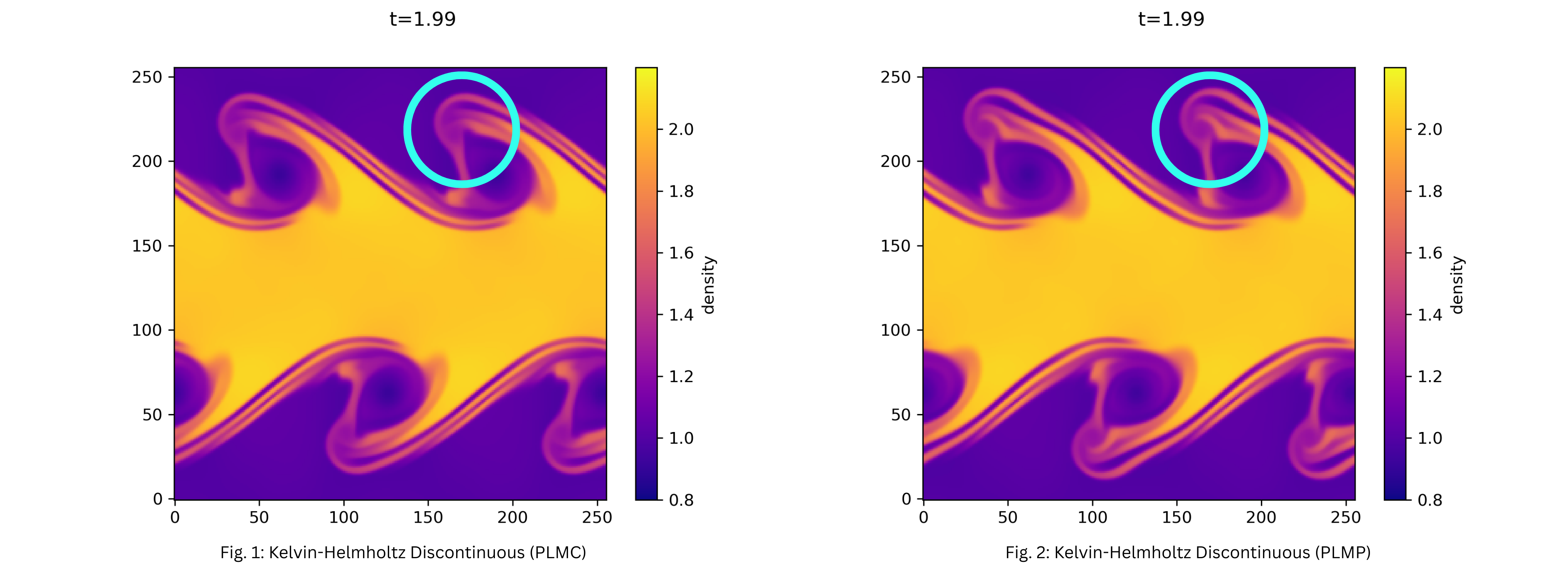
In this example, we are comparing the final snapshot of the Kelvin-Helmholtz Discontinuous tests using both PLMC and PLMP. We see that while the PLMP reconstruction is slightly more diffusive than the PLMC as the PLMC method has a higher accuracy for instabilities. The overall result, however, differs only minorly and an accurate result can be achieved with the PLMP reconstruction.
PLMP vs PPMP
1D Example:
This movie shows the evolution of the square wave test with both the PLMP and PPMP reconstructions. As opposed to the initial comparison of the PLMP and PLMC reconstructions, there is a more significant difference in these simulations. The PPMP simulation maintains steeper edges of the curve whereas the PLMP falls off more gradually at the edges.
2D Example:
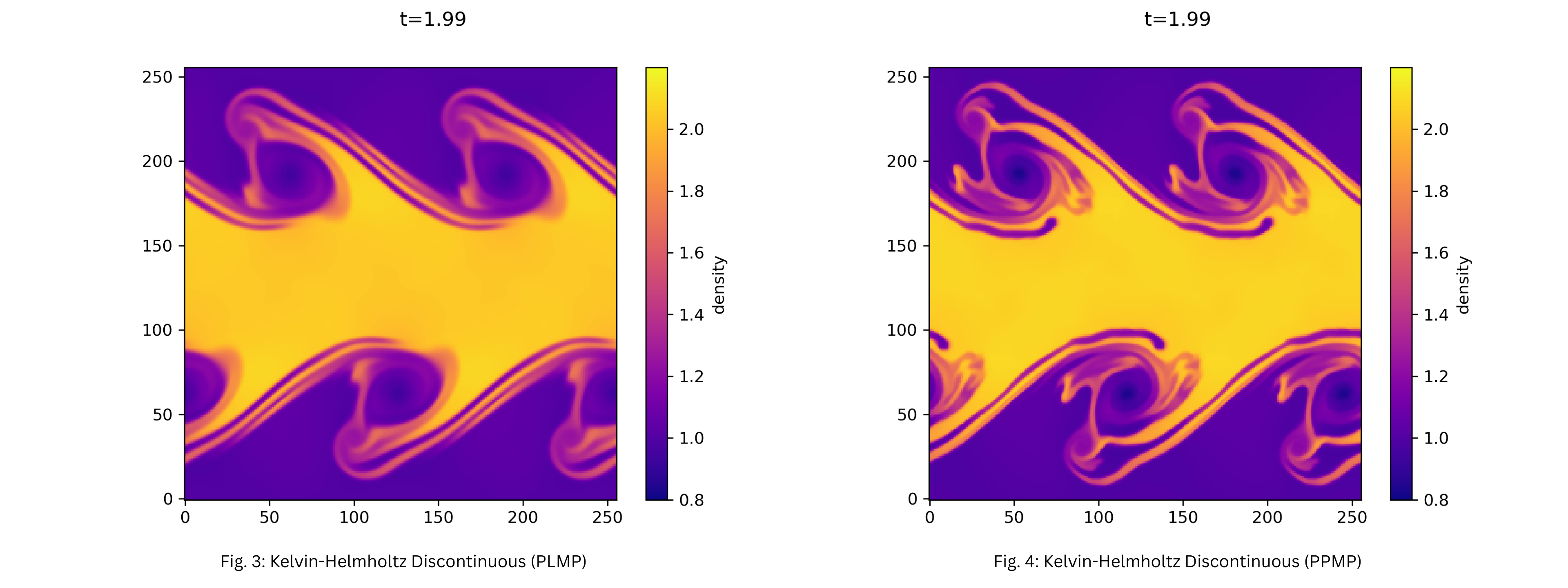
In this example, we are comparing the final snapshot of the Kelvin-Helmholtz Discontinuous tests using both PLMP and PPMP. The difference between these two methods is much more apparent than what is observed between the PLMC and PLMP methods. For this instability, although the general shape of the fluids remain the same, the PPMP result is more evolved within the same time constraint.